Motivation
I’ve been a long-time user of Xterm. I tried to switch to other terminal emulators several times because of Xterm’s broken Unicode support, especially regarding glyphs/emojis and multi-font substitution. These glyphs are part of many modern CLI tools and are often printed as blank squares in Xterm. More recently, I attempted to switch again, but every time I try, I’m discouraged by the additional latency added during typing. I’m not a super-fast typist. I average about 80 WPM for normal text with bursts for common terminal commands of up to 120 WPM. The text appears in the terminal, of course, but not as quickly as I would like. There is a noticeable delay, especially when comparing something like Xterm to xfce4-terminal. I’ve placed some hope in the recent development of GPU-accelerated terminals, e.g., wezterm, but it still felt as slow as xfce4-terminals. When I read the benchmarks, they often show how fast it can print a gigabyte text file to stdout, but honestly, this is something I’m not so interested in for everyday use. I found some other interesting benchmarks regarding terminal latency, but there were always some terminal emulators missing for which I would like to know the result, or the results were slightly outdated.
Benchmark
For the benchmark, I used Typometer[1], a tool designed to measure and analyze the latency of various applications that have text input. The test does not include keyboard latency or display latency, as Typometer emulates the keystrokes in software, and the screen capture is also in software, not via a physical camera in front of the screen. Hence, you can expect additional latency from the hardware, and these measurements represent only the latency that originates from the software stack. All versions should be either the latest stable version available via Arch Linux at the time of writing or the latest master commit. All tests were conducted on the same machine, a T14 Gen 1 (AMD Ryzen 7 PRO 4750U) with Arch Linux and Xorg (21.1.11-1).
Results
| Terminal Emulator | Min | Max | Avg | Stddev |
|---|---|---|---|---|
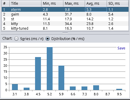
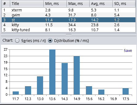
| xterm (389-1) | 2.8 | 9.8 | 5.3 | 1.1 |
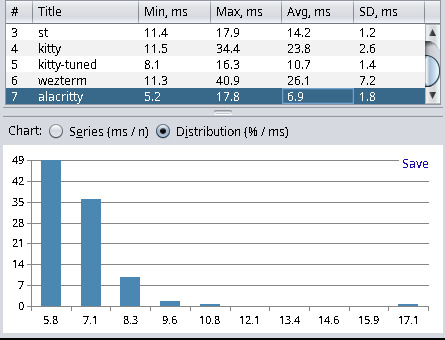
| alacritty (0.13.1-1) | 5.2 | 17.8 | 6.9 | 1.8 |
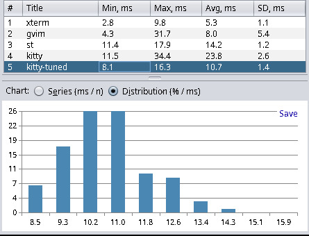
| kitty-tuned (0.31.0-1) | 8.1 | 16.3 | 10.7 | 1.4 |
| zutty (0.14-2) | 7.4 | 16.4 | 11.2 | 1.6 |
| st (master 95f22c5) | 11.4 | 17.9 | 14.2 | 1.2 |
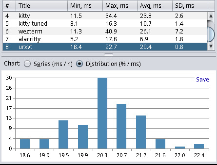
| urxvt (9.31-4) | 18.4 | 22.7 | 20.4 | 0.8 |
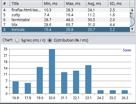
| konsole (24.02.0-1) | 16.4 | 26.8 | 20.7 | 2.2 |
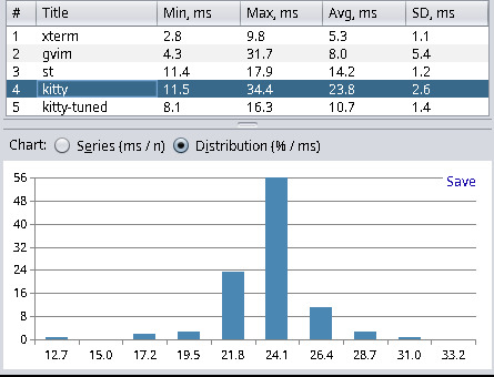
| kitty (0.31.0-1) | 11.5 | 34.4 | 23.8 | 2.6 |
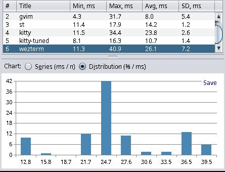
| wezterm (20230712.072601) | 11.3 | 40.9 | 26.1 | 7.2 |
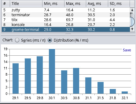
| gnome-terminal (3.50.1-1) | 29.0 | 32.3 | 30.2 | 0.8 |
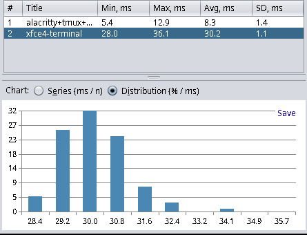
| xfce4-terminal (1.1.1-2) | 28.0 | 36.1 | 30.2 | 1.1 |
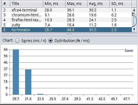
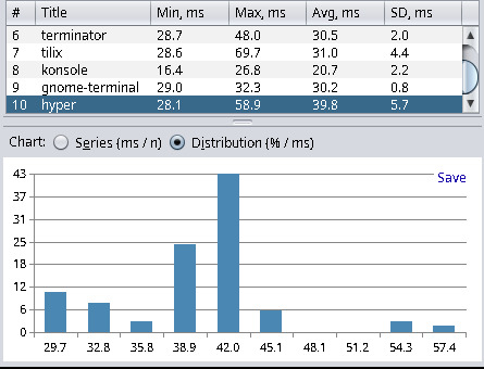
| terminator (2.1.3-3) | 28.7 | 48.0 | 30.5 | 2.0 |
| tilix (1.9.6-3) | 28.6 | 69.7 | 31.0 | 4.4 |
| hyper (v3.4.1) | 28.1 | 58.9 | 39.8 | 5.7 |
Xterm yields the best results, and Hyper (a web-based terminal) has the worst results. This has met my expectations and matched the results from other blog posts. Hyper, with about 40ms latency, is not as bad as I thought. However, anything with more than 20ms I consider a noticeable delay, and everything below 10ms is fast enough for my needs. I find it quite interesting that kitty can be tuned to be more than twice as fast in terms latency. For kitty tuned I used the following settings:
# 150 FPSrepaint_delay 8# Remove artificial input delayinput_delay 0# turn off vsyncsync_to_monitor noI gathered these settings from another blog post about terminal latency[2], which is worth reading. Please note that the results in this blog post are not comparable with the results shown here because the author used a camera to measure the latency, which also includes the latency of the monitor.
I’ve also tested the following applications:
| Application | Min | Max | Avg | Stddev |
|---|---|---|---|---|
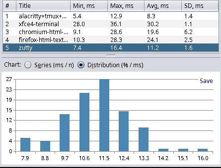
| gvim (9.1.0000-1) | 4.3 | 31.7 | 8.0 | 5.4 |
| alacritty+tmux+neovim (0.13.1-1+3.3_a-7+0.9.5-2) | 5.4 | 12.9 | 8.3 | 1.4 |
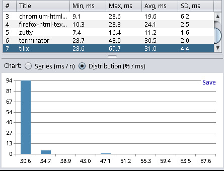
| chromium (120.0.6099.216-1) | 9.1 | 28.6 | 19.6 | 6.2 |
| firefox (121.0.1-1) | 10.3 | 28.3 | 24.1 | 2.5 |
| Visual Studio Code (1.87.2-1) | 26.3 | 36.7 | 31.2 | 3.3 |
As we can see, the latency for Neovim inside tmux inside Alacritty (8.3 ms) is not much higher than just Alacritty (6.9 ms). Hence, tmux and Neovim add only about 1.4 milliseconds of latency, which is quite acceptable. We can also see that the latency of an HTML text area in Chromium or Firefox is more than double the Alacritty latency. So, if you often write in applications like Teams, then there is probably not much you can do about it, other than accept about 20 milliseconds of delay for typing. And you are also out of luck in terms of latency if your favorite code editor of choice is Visual Studio Code, as this editor clocks in with a 31.2 ms delay before any hardware latency considerations.
Conclusion
I’m quite satisfied with the results, especially now that I have found a decent alternative to Xterm, which has only 1.7 ms more latency - Alacritty. I’ve seen benchmarks in the past that measured higher values for Alacritty. Hence, I think the terminal latency has improved over time due to complaints on GitHub[3] that caught some attention from the maintainers (there’s also my thumbs up on that issue). For now, I will migrate my configs from Xterm to Alacritty and report back in the form of another blog post in case there are any issues.
Update: March 17, 2024
One of the contributors[4] to the st terminal emulator reached out to me and mentioned the possibility of configuring and recompiling st for lower latency. One might ask why the latency settings are not zero altogether for the smallest possible delay. Here’s the answer by avih:
Generally speaking, there's a tradeoff between latency and throughput/flicker.The smaller the latency, the worse the throughput is (e.g. in cat huge.txt) because the terminal has to render more frequently, and the more flicker-prone it becomes, for instance when the terminal updates the screen before the application completed its “output batch” - which then requires another screen update once the output batch is complete, e.g. when holding page-down in auto-repeat in vim or less.
This behavior is not unique to st, but what is unique to st is that it’s configurable, and can be adaptive.
By default it’s adaptive between 8 and 32 ms, and tries to draw as soon as possible after the application-output batch completes, i.e. the terminal input becomes idle.
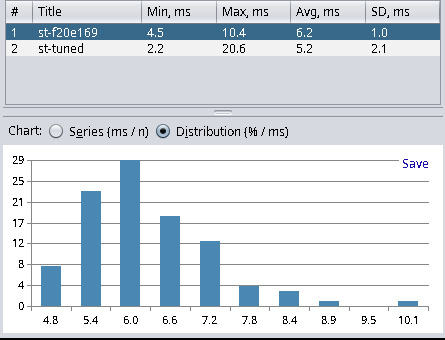
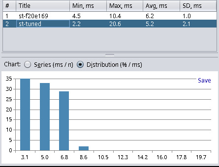
In response to this blog post, the default minlatency setting of st has now changed from 8 milliseconds to 2 to offer a smaller default latency for all users. I’ve chosen to rerun the tests, of course. Here are the new results:
| Terminal Emulator | Min | Max | Avg | Stddev |
|---|---|---|---|---|
| st (master f20e169) | 4.5 | 10.4 | 6.2 | 1.0 |
| st (custom f20e169) | 2.2 | 20.6 | 5.2 | 2.1 |
With the new commits, the master branch of st is now placed second, behind xterm and before Alacritty. However, if we custom-tune the settings for the lowest latency possible I chose minlatency = 0 and maxlatency = 1 then we have a new winner. Applying this custom tuning results in an average latency of 5.2 ms, which is 0.1 ms lower than xterm, and that’s with having a much more sane terminal without legacy cruft.


