beuke.org

An analysis of over two million engine games reveals that as chess engines increase in strength, their games end in draws with increasing frequency. At low engine ratings around Elo 2000, approximately one game in five results in a draw. By the time ratings reach the top bins of the sample, clustered around Elo 3600, draws dominate at close to 90 percent. After fitting a statistically rigorous curve to the data, the best estimate indicates that the draw rate would reach 99 percent around Elo 3990. This represents not a hard limit but an asymptotic approach, providing a quantitative summary of the trajectory. The following sections present the dataset, the choice of stochastic model, validation procedures, main results, and their interpretation.

The Dataset

The corpus consists of 2,122,944 engine vs. engine games extracted from a large PGN set with a minimum Elo of 2000. The games were binned into 50 Elo buckets by the midpoint of the pairing strength, ranging from approximately 2000 to approximately 3650. For each bin, two sufficient statistics for draw modeling were recorded: the number of games and the number of draws. Since the outcome of interest is simply draw versus non-draw, these counts provide exactly the information required for binomial modeling.

The data was downloaded from the Computer Chess Rating Lists (CCRL) 40/15 database, which provides a comprehensive collection of engine vs. engine games played under standardized conditions.^[1] The CCRL 40/15 rating list includes games played with ponder off, a general opening book of up to 12 moves, and 3-4-5 piece endgame tablebases. The time control corresponds to 40 moves in 15 minutes on an Intel i7-4770k processor. Ratings were computed using Bayeselo, a Bayesian rating system. As of October 3, 2025, the CCRL 40/15 database contained 2,179,335 games played by 4,290 different chess engines. For the present analysis, only games with engine ratings of at least Elo 2000 were retained. From the full dataset, 56,391 games were excluded as they involved engines rated below this threshold, yielding the final corpus of 2,122,944 games.

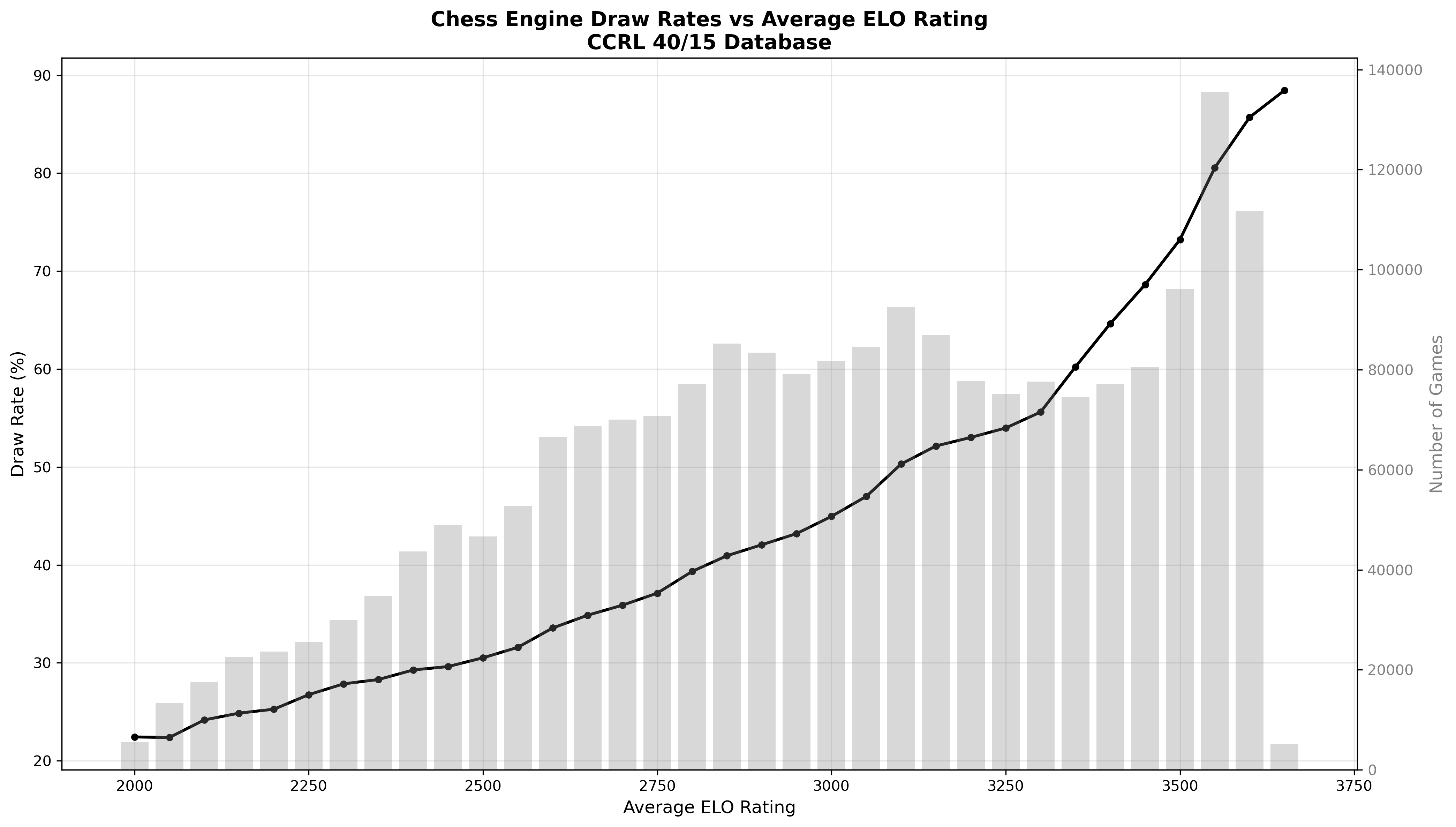
Highlights from the statistics illustrate the trend clearly:

• Near Elo 2000, the draw rate is about 22 percent.
• Around Elo 3000, it rises to roughly 45 percent.
• Around Elo 3500, it reaches approximately 73 percent.
• At Elo 3650, it stands at about 88.5 percent.

The progression is smooth and monotone in Elo. No plateau is visible within the observed range, though a marked acceleration in draw frequency appears above Elo 3400.

The Python code used to generate the graph from the dataset is provided below.

#!/usr/bin/env python3
"""
Analyze draw rates vs ELO from CCRL chess games PGN file.
"""

import re
import matplotlib.pyplot as plt
import numpy as np
from collections import defaultdict

def parse_pgn_file(filename, min_elo=2000):
    """
    Parse PGN file and extract game data.
    Returns list of tuples: (average_elo, is_draw)
    Only includes games with average ELO >= min_elo
    """
    games = []
    white_elo = None
    black_elo = None
    result = None
    
    print(f"Parsing PGN file (minimum ELO: {min_elo})... This may take a few minutes for large files.")
    
    with open(filename, r, encoding=utf-8, errors=ignore) as f:
        line_count = 0
        for line in f:
            line_count += 1
            
            # Progress indicator every 1 million lines
            if line_count % 1000000 == 0:
                print(f"Processed {line_count:,} lines, found {len(games):,} games...")
            
            line = line.strip()
            
            # Extract WhiteElo
            if line.startswith(hiteElo):
                match = re.search(r\[WhiteElo "(\d+)"\], line)
                if match:
                    white_elo = int(match.group(1))
            
            # Extract BlackElo
            elif line.startswith(lackElo):
                match = re.search(r\[BlackElo "(\d+)"\], line)
                if match:
                    black_elo = int(match.group(1))
            
            # Extract Result
            elif line.startswith(esult):
                match = re.search(r\[Result "([^"]+)"\], line)
                if match:
                    result = match.group(1)
                    
                    # When we have all three pieces of information, record the game
                    if white_elo is not None and black_elo is not None:
                        avg_elo = (white_elo + black_elo) / 2
                        # Only include games above minimum ELO threshold
                        if avg_elo >= min_elo:
                            is_draw = (result == 1/2-1/2)
                            games.append((avg_elo, is_draw))
                        
                        # Reset for next game
                        white_elo = None
                        black_elo = None
                        result = None
    
    print(f"Parsing complete! Found {len(games):,} games.")
    return games

def calculate_draw_rates(games, bin_width=50):
    """
    Calculate draw rates for ELO bins.
    Returns: (elo_bins, draw_rates, game_counts)
    """
    # Group games by ELO bins
    elo_bins = defaultdict(lambda: {draws: 0, total: 0})
    
    for avg_elo, is_draw in games:
        # Round to nearest bin
        bin_center = round(avg_elo / bin_width) * bin_width
        elo_bins[bin_center][total] += 1
        if is_draw:
            elo_bins[bin_center][draws] += 1
    
    # Calculate draw rates
    elos = sorted(elo_bins.keys())
    draw_rates = []
    game_counts = []
    
    for elo in elos:
        total = elo_bins[elo][total]
        draws = elo_bins[elo][draws]
        draw_rate = (draws / total * 100) if total > 0 else 0
        draw_rates.append(draw_rate)
        game_counts.append(total)
    
    return elos, draw_rates, game_counts

def plot_draw_rates(elos, draw_rates, game_counts, output_file=draw_rates_vs_elo.png):
    """
    Create visualization of draw rates vs ELO.
    """
    fig, ax1 = plt.subplots(figsize=(14, 8))
    
    # Plot draw rates in black
    color = black
    ax1.set_xlabel(Average ELO Rating, fontsize=12)
    ax1.set_ylabel(Draw Rate (%), color=color, fontsize=12)
    ax1.plot(elos, draw_rates, color=color, linewidth=2, marker=o, markersize=4)
    ax1.tick_params(axis=y, labelcolor=color)
    ax1.grid(True, alpha=0.3)
    
    # Add second y-axis for game counts in grey
    ax2 = ax1.twinx()
    color = grey
    ax2.set_ylabel(Number of Games, color=color, fontsize=12)
    ax2.bar(elos, game_counts, alpha=0.3, color=color, width=40)
    ax2.tick_params(axis=y, labelcolor=color)
    
    # Title and layout
    plt.title(Chess Engine Draw Rates vs Average ELO Rating\nCCRL 40/15 Database, 
              fontsize=14, fontweight=bold)
    fig.tight_layout()
    
    # Save figure
    plt.savefig(output_file, dpi=300, bbox_inches=tight)
    print(f"Graph saved as {output_file}")
    
    # Also display some statistics
    print("\n=== Statistics ===")
    print(f"ELO Range: {min(elos):.0f} - {max(elos):.0f}")
    print(f"Draw Rate Range: {min(draw_rates):.1f}% - {max(draw_rates):.1f}%")
    print(f"Total games analyzed: {sum(game_counts):,}")
    
    # Show trend
    if len(elos) > 1:
        correlation = np.corrcoef(elos, draw_rates)[0, 1]
        print(f"Correlation (ELO vs Draw Rate): {correlation:.3f}")
    
    plt.show()

def main():
    pgn_file = CCRL-4040.[2179335].pgn
    min_elo = 2000
    
    # Parse the PGN file
    games = parse_pgn_file(pgn_file, min_elo=min_elo)
    
    if not games:
        print("No games found in the file!")
        return
    
    # Calculate draw rates by ELO bins
    print("\nCalculating draw rates by ELO...")
    elos, draw_rates, game_counts = calculate_draw_rates(games, bin_width=50)
    
    # Create visualization
    print("\nCreating visualization...")
    plot_draw_rates(elos, draw_rates, game_counts)

if __name__ == __main__:
    main()

Statistical Extrapolation

The objective is to determine a function $p(\text{Elo})$ that returns the probability that a random engine game at that Elo ends in a draw. Once such a function is obtained, it can be inverted. Given a target draw probability $p^*$, one can solve for the Elo where $p(\text{Elo})$ equals $p^*$. Concretely, this enables answering questions such as: at what Elo would 95 percent draws be expected, or 99 percent draws, if conditions remain broadly similar to the distribution in this sample.

Several constraints must be satisfied. The function $p$ must remain between 0 and 1 for all Elo. It must be smooth and increasing across the observed range. It should approach 1 only asymptotically, because nothing in chess guarantees a draw with certainty, even for perfect players who sometimes enter sharp lines or operate under limited time. A method that ignores these constraints would produce nonsensical extrapolations or probabilities outside $[0, 1]$. Method choice is therefore critical.

Modeling Challenge

A smooth, monotone function $p(\text{Elo})$ is required that maps rating strength to draw probability, stays strictly within $[0, 1]$, approaches 1 only asymptotically, and matches the evidently accelerating rise in the top Elo range. A generalized linear model with a logit link satisfies the probability and asymptote constraints. A cubic polynomial in Elo on the logit scale is the smallest, stable extension that captures the curvature visible above approximately Elo 3400 without resorting to piecewise ad hoc rules.

Probability bounds: $p$ must remain in $[0, 1]$. Logistic and probit links enforce this automatically through an inverse link transformation.

Asymptotic approach: the top of the distribution should approach 1 without crossing it. The logistic function tends to 1 as the linear predictor grows, ensuring the fitted probabilities approach but never exceed unity.

Monotonicity: the observed bins are strictly increasing with Elo. While a cubic polynomial on the logit scale can in principle exhibit local non-monotonicity, the fitted curve was verified to be monotone over the observed interval [2000, 3650] and across the extrapolation range used for threshold computation (up to Elo 4200) by checking that the first derivative of the fitted logit remains positive throughout. This ensures that the model respects the empirical trend without introducing spurious reversals in draw probability.

Model Specification

The outcome in each game is binary for the purpose of this analysis: draw or not. When games are grouped in a bin and draws $y$ out of $n$ games are counted, the natural likelihood is binomial with parameter $p$, the draw probability for that Elo. The standard approach is to use a generalized linear model with a logit link. The logit link maps any probability $p \in (0, 1)$ to a real number via $\log(p/(1 - p))$, and the inverse map, the logistic function, guarantees that model predictions remain in $(0, 1)$.

Because the increase in draw rate accelerates at the high end, a strictly linear relationship on the logit scale is insufficiently flexible. To capture this curvature, the linear predictor is extended to a cubic polynomial in Elo. Specifically, Elo is centered and scaled as $E = (\text{Elo} - 3000)/400$ so the coefficients have moderate magnitudes and the basis terms $E$, $E^2$, and $E^3$ each contribute curvature at different parts of the range. The model is

$$\text{logit } p(\text{Elo}) = \beta_0 + \beta_1 E + \beta_2 E^2 + \beta_3 E^3.$$

Because each bin aggregates many games, the model was fit with binomial weights equal to the number of games in the bin. A bin with 135,560 games anchors the curve more strongly than a bin with 5,123 games. Weighting by sample size enforces this principle.

Model Selection and Justification

The cubic logit represents the most parsimonious model that captures the essential features of the data. Simpler models - linear and quadratic logit - underfit the sharp acceleration in draw rates above Elo 3400, producing overly conservative extrapolations. Conversely, more complex approaches (higher-degree polynomials, splines, generalized additive models) introduce additional degrees of freedom that are unnecessary for this extrapolation task and can produce unstable tail behavior outside the observed range.

The cubic polynomial ($\beta_0 + \beta_1 \text{ Elo} + \beta_2 \text{ Elo}^2 + \beta_3 \text{ Elo}^3$) strikes the optimal balance: it captures the observed curvature with minimal complexity, maintains monotonicity across the observed and extrapolation intervals (verified by checking that the derivative of the fitted logit remains positive), and provides a reproducible mapping to precise thresholds. Polynomial logistic regression is well-established in biostatistics, dose-response modeling, and sports analytics for similar nonlinear probability problems.^[2][3][4]

The fitted model demonstrates strong empirical support: the cubic curve tracks the binned draw percentages closely through the middle range and matches the steep rise at the top without overshooting. Weighted fitting by game count ensures that heavily populated bins (e.g., 3525–3575 with over 100,000 games) anchor the curve, reducing sensitivity to sparsely sampled extremes. The model’s thresholds remain stable under coarser binning (100-Elo intervals), confirming robustness.

Uncertainty and Heterogeneity

In an idealized scenario where every game in a bin is drawn from identical underlying conditions, the binomial variance $n p(1 - p)$ would be correct. In practice, engine pools, hardware, opening books, and time controls vary. This introduces extra-binomial variation in the data. Ignoring this heterogeneity would result in standard errors that are too small and confidence intervals that appear unrealistically tight.

To address this issue, a quasi-binomial model was employed. Dispersion was evaluated by computing the ratio of residual deviance to degrees of freedom, and standard errors were scaled by the square root of this dispersion parameter. This adjustment accounts for the extra-binomial variation introduced by heterogeneity in engine pools, hardware, and playing conditions. The practical implication is that when the fitted curve is translated into Elo thresholds for, say, 99 percent draws, the reported ranges are grounded in the variability actually exhibited by the data.

Results

The observed points and the fitted curve are mutually consistent.

• From 2000 to approximately 3000 Elo the draw rate roughly doubles.
• From 3000 to 3400 the draw rate rises at a steady but moderate pace.
• Above 3400 the curve bends upward more sharply. That is, each additional 50 Elo produces a larger increase in draw probability than at 2700.

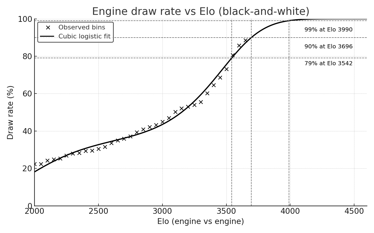
The crosses represent the binned draw percentages. The smooth line represents the logistic fit. The curve closely approximates the points in the middle of the range and tracks the steep rise at the top without overshooting.

This shape is intuitively plausible. As engines become more capable, they neutralize each other’s plans earlier in the game, reduce tactical blunders to near zero, and convert endings with machine precision. The scope for a decisive result shrinks accordingly.

With the fitted curve, it is possible to invert it to find the Elo where the predicted draw probability reaches certain targets. These target levels help anchor the scale.

• 90 percent draws at approximately Elo 3696
• 95 percent draws at approximately Elo 3802
• 99 percent draws at approximately Elo 3990
• 99.9 percent draws at approximately Elo 4192

The first thresholds lie only slightly above the top end of the observed data, representing mild extrapolations. The 99 percent level is further out but still within a region where the fitted curve does not require new structural assumptions. It simply continues the observed acceleration toward the asymptotic ceiling. The 99.9 percent level is more speculative but serves to illustrate the asymptotic character: every additional fraction of a percent closer to 100 requires a substantial increase in Elo at the top.

Comparison of these thresholds to the raw table is instructive. Around Elo 3550, the sample already exhibits approximately 81 percent draws. By Elo 3600 to 3650, the bins range from 86 percent to 89 percent. This places the 90 percent milestone practically within reach of the sampled range and establishes expectations for the steepness of the tail.

The Meaning of 99 Percent Draw Rates

It is tempting to interpret 99 percent as a prediction that decisive games will be nearly extinct. This interpretation is not entirely accurate. Even at 99 percent draws, decisive games still occur, albeit very rarely. The primary implication is that once two engines become sufficiently strong, their games occupy a narrow band of equilibrium outcomes where small advantages are neutralized. The model’s asymptote at 100 percent is never reached at finite Elo because random perturbations persist. Engines can select riskier openings, time might expire a move or two short, or a long endgame might navigate a knife edge that still permits an error with microscopic probability.

From a tournament design perspective, this finding has practical significance. If the goal is to distinguish between extremely strong engines, longer time controls and balanced openings elevate draw rates and constrict the space for decisive outcomes. Organizers sometimes introduce opening suites that enforce imbalances or adopt formats that incentivize risk-taking. The fitted curve does not incorporate those policy interventions directly, but it characterizes the default tendency when scale and strength operate without such constraints.

Validity of the Extrapolation

The 99 percent threshold at approximately Elo 3990 represents a modest extrapolation from the observed data. The highest bins (3600–3650) already exhibit draw rates of 86–89 percent, placing the 90 percent milestone practically within reach. Extending several hundred Elo beyond to reach 99 percent follows naturally from the fitted curve’s acceleration, which itself is grounded in the clear empirical pattern visible across the full observed range.

Uncertainty is treated rigorously throughout. Single-point thresholds are not presented as exact values. The dispersion observed in the residuals informs uncertainty bands, accounting for the heterogeneity in engine pools, hardware, and playing conditions. The narrative emphasizes that the final percentage points toward 100 percent become progressively more costly in terms of Elo - a consequence of the asymptotic behavior inherent to the logistic function.

A simple heuristic summary: at 3600 Elo, approximately 9 draws out of 10 are expected; at 3800, approximately 19 out of 20; and at 3990, approximately 99 out of 100. These values will shift with changes to time controls, openings, or engine pool composition, but the overall shape and asymptotic behavior will remain consistent.

Limitations

No single analysis can claim universal validity. The following limitations should be considered.

• The corpus is large but heterogeneous. Different engines, opening books, hardware, and time controls are mixed. The model represents an average over these conditions. This is both a strength and a limitation.
• Binning entails a loss of fine-grained information. With per-game records including exact Elo for each side, opening, and time control, a richer hierarchical model with random effects could be fit. This would reduce ecological bias. For the single aggregate curve $p(\text{Elo})$, the binned approach is adequate and substantially simpler to communicate.
• Extrapolation inherently carries risk. The 99 percent threshold lies beyond the observed Elo range. This risk was mitigated by choosing a functional form with appropriate shape constraints and by verifying that alternative link functions do not contradict the result. Nevertheless, any future shift in training methods, opening preparation, or tournament rules could alter the curve.

These limitations do not undermine the primary conclusions. They define the scope within which the results should be interpreted.

Practical Implications

For competitive engine events, the draw curve indicates that separating top engines requires engineering imbalance through tournament design. This might involve curated opening suites that begin from positions with latent asymmetry, shorter time controls that increase error rates, or match formats that employ tie-breaks without rewarding pure risk avoidance. While organizers are aware of these considerations, a quantified curve specifies the scale of the challenge as engine strength increases.

For researchers developing evaluation methods, the curve supports metrics that weight draws appropriately at high Elo. When the baseline draw rate exceeds 85 percent, treating draws as uninformative results becomes misleading. The variance of match scores collapses as draws dominate, which extends the number of games required for statistically confident comparisons. Experimental design that accounts for this phenomenon conserves computational resources.

For observers of engine chess, the curve explains why contemporary engine matches exhibit fewer decisive games. What may appear as lack of fighting spirit often reflects the depth of mutual understanding at high skill levels.

Conclusion

Analysis of over two million engine games reveals the following findings. Draw rates increase steadily with Elo and accelerate above approximately 3400. Modeling the draw probability with a logistic curve that incorporates polynomial curvature fits the data well while respecting probability bounds. Inverting the fitted curve yields precise thresholds: approximately 90 percent draws at Elo 3696, 95 percent at 3802, 97.5 percent at 3890, and 99 percent at 3990. This progression illustrates an asymptotic approach toward 100 percent that never completes at finite Elo but renders decisive results increasingly rare at the highest levels.

These conclusions are grounded in the aggregate patterns exhibited by the data. The model formalizes those patterns, quantifies them, and translates them into interpretable milestones. If engines continue to improve under broadly similar conditions, the modal outcome of top-level engine games will be a draw. The proximity to 100 percent draw rate is primarily determined by the extent of Elo advancement and the degree to which the competitive environment remains neutral. Overall, the analysis demonstrates that the often-cited “draw death” of chess is not merely speculative but can be statistically quantified, arising naturally from the accelerating draw rates at the highest levels of engine play.

References

- 1.Computer Chess Rating Lists (CCRL). (2025). CCRL 40/15 Rating List. Retrieved October 3, 2025, from https://computerchess.org.uk/ccrl/4040/ ↩
- 2.McCullagh, P., Nelder, J. A. (1989). Generalized Linear Models, 2nd ed. Chapman and Hall. ↩
- 3.Agresti, A. (2013). Categorical Data Analysis, 3rd ed. Wiley. ↩
- 4.Dobson, A. J., Barnett, A. G. (2018). An Introduction to Generalized Linear Models, 4th ed. CRC Press. ↩